Pharmacokinetics

Dose-Exposure

“What the body does to the drug”

Executive summary

Pharmacokinetics (PK) asks a single question:

“Given an input (dose & regimen), what exposure (concentration-time profile) will the body create?”

This page is your quick-reference for that mapping. It is organised as follows:

Section	What you get	Key take-aways
Therapeutic window	Where efficacy ⇢ safety overlap	Target Cmin and Cmax
Single-dose kinetics	IV bolus + oral equations	How Vd and ke shape curves
Repeated/continuous input	Multiple-dose & infusion profiles	Why accumulation ratio (Rac) matters
Equations at a glance	One-liner table of canonical PK formulae	Copy-paste cheatsheet
Deep dives	Absorption · Distribution · Elimination	Mechanistic levers behind each parameter

Use the overview to choose the right regimen, then jump to the deep-dive pages when you need mechanism-level detail.

Key symbols and canonical equations

Table 1: Pharmacokinetic symbols

Symbol	Description
$\mathrm{Dose}$	Dose
$\tau$	Dosing interval (interdose interval)
$\mathrm{CL}$	Clearance
${\mathrm{V}}_{\mathrm{d}}$	Volume of distribution
${\mathrm{k}}_{\mathrm{e}}$	Elimination rate constant
${\mathrm{k}}_{\mathrm{a}}$	Absorption rate constant
$\mathrm{F}$	Bioavailability
${\mathrm{R}}_{\mathrm{in}}$	Infusion rate
$T_{\text{inf}}$	Duration of infusion
${\mathrm{C}}_{\mathrm{pl}}$	Plasma concentration
${\mathrm{R}}_{\mathrm{ac}}$	Accumulation ratio

Clearance (CL)

$$\begin{array}{}\text{(1)}& \mathrm{CL}=\frac{\mathrm{Dose}\times \mathrm{F}}{{\mathrm{AUC}}_{0\mathrm{-}\mathrm{\infty }}}={\mathrm{k}}_{\mathrm{e}}\times {\mathrm{V}}_{\mathrm{d}}\end{array}$$

Therapeutic window

tibble::tibble(
  time = c(0, 0.5, 1, 2, 4, 6, 8, 12), # h
  conc = c(0, 14, 12, 9, 6, 4, 3, 0) # mg/L (example)
) |>
ggplot2::ggplot(ggplot2::aes(time, conc)) +
  ggplot2::annotate( # shaded window
    "rect",
    xmin = -Inf,
    xmax = Inf,
    ymin = 3,
    ymax = 10,
    alpha = 0.08,
    fill = "forestgreen"
  ) +
  ggplot2::geom_line(linewidth = 1) +
  ggplot2::geom_hline(yintercept = 3, linetype = "dashed") + # MEC
  ggplot2::geom_hline(yintercept = 10, linetype = "dashed") + # MTC
  ggplot2::labs(
    x = "Time (h)",
    y = "Concentration (mg/L)"
  ) +
  ggplot2::annotate( # labels
    "text",
    x = 11.5,
    y = 10.4,
    hjust = 1,
    label = "Safety threshold",
    size = 3
  ) +
  ggplot2::annotate(
    "text",
    x = 11.5,
    y = 3.4,
    hjust = 1,
    label = "Efficacy threshold",
    size = 3
  ) +
  ggplot2::theme_minimal()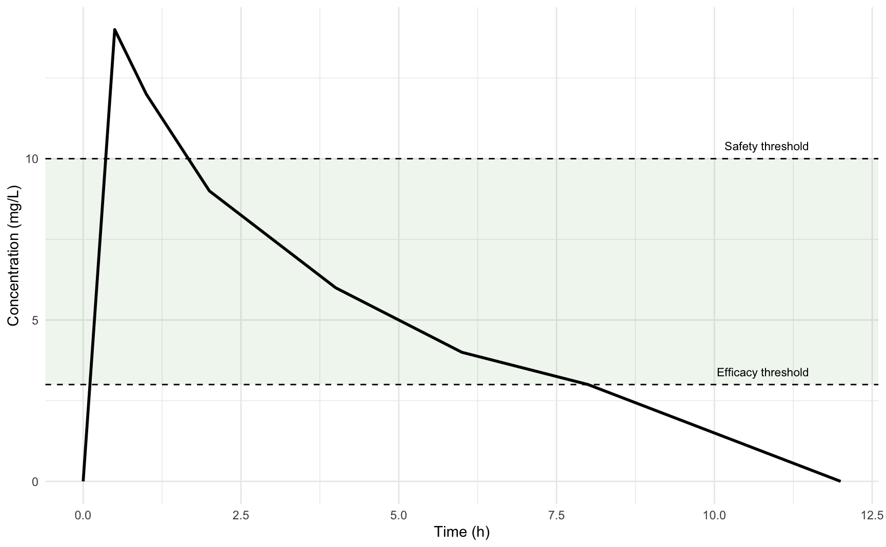

Figure 1: Concentration–time profile and the therapeutic window.

Single-dose kinetics

Intravenous bolus

Single i.v. dose

Initial concentration Equation 2.

$$\begin{array}{}\text{(2)}& {\mathrm{C}}_0=\frac{\mathrm{Dose}}{{\mathrm{V}}_{\mathrm{d}}}\end{array}$$

Plasma concentration Equation 3.

$$\begin{array}{}\text{(3)}& \mathrm{C}(t)={\mathrm{C}}_0\times e^{-{\mathrm{k}}_{\mathrm{e}}\times t}\end{array}$$

Multiple i.v. doses

$${\mathrm{C}}_n(t)=\frac{\mathrm{Dose}}{{\mathrm{V}}_{\mathrm{d}}}\times \frac{(1-e^{-n\times {\mathrm{k}}_{\mathrm{e}}\times \tau })}{(1-e^{-{\mathrm{k}}_{\mathrm{e}}\times \tau })}\times e^{-{\mathrm{k}}_{\mathrm{e}}\times t}$$

at peak: $t=0$; at steady state $\mathrm{n}\to \mathrm{\infty }$; at trough: $t=\tau$

$$\begin{array}{}\text{(4)}& {\mathrm{C}}_{\text{max, ss}}=\frac{\mathrm{Dose}}{\mathrm{V}}\times \frac{1}{(1-e^{-{\mathrm{k}}_{\mathrm{e}}\tau })}\end{array}$$

$$\begin{array}{}\text{(5)}& {\mathrm{C}}_{\text{min, ss}}={\mathrm{C}}_{\text{max, ss}}\times e^{-{\mathrm{k}}_{\mathrm{e}}\times \tau }\end{array}$$

Plasma concentration Equation 6.

$$\begin{array}{}\text{(6)}& \mathrm{C}(t)={\mathrm{C}}_{\max }\times e^{-{\mathrm{k}}_{\mathrm{e}}\times t}\end{array}$$

Peak Equation 7.

$$\begin{array}{}\text{(7)}& {\mathrm{C}}_{\max }=\frac{{\mathrm{C}}_0}{1-e^{-{\mathrm{k}}_{\mathrm{e}}\times \tau }}\end{array}$$

Trough Equation 8.

$$\begin{array}{}\text{(8)}& {\mathrm{C}}_{\min }={\mathrm{C}}_{\max }\times e^{-{\mathrm{k}}_{\mathrm{e}}\times \tau }\end{array}$$

Average concentration (steady state) Equation 9.

$$\begin{array}{}\text{(9)}& {\overline{\mathrm{C}}}_{\text{pl, ss}}=\frac{\mathrm{Dose}}{\mathrm{CL}\times \tau }\end{array}$$

Oral administration

Single p.o. dose

Plasma concentration Equation 10.

$$\begin{array}{}\text{(10)}& \mathrm{C}=\frac{\mathrm{F}\times \mathrm{Dose}\times {\mathrm{k}}_{\mathrm{a}}}{{\mathrm{V}}_{\mathrm{d}}({\mathrm{k}}_{\mathrm{a}}-{\mathrm{k}}_{\mathrm{e}})}(e^{-{\mathrm{k}}_{\mathrm{e}}\times t}-e^{-{\mathrm{k}}_{\mathrm{a}}\times t})\end{array}$$

Time of maximum concentration Equation 11.

$$\begin{array}{}\text{(11)}& t_{\text{max}}=\frac{\ln \left({\mathrm{k}}_{\mathrm{a}}/{\mathrm{k}}_{\mathrm{e}}\right)}{{\mathrm{k}}_{\mathrm{a}}-{\mathrm{k}}_{\mathrm{e}}}\end{array}$$

Multiple p.o. doses

Plasma concentration Equation 12.

$$\begin{array}{}\text{(12)}& \mathrm{C}=\frac{\mathrm{F}\times \mathrm{Dose}\times {\mathrm{k}}_{\mathrm{a}}}{{\mathrm{V}}_{\mathrm{d}}({\mathrm{k}}_{\mathrm{a}}-{\mathrm{k}}_{\mathrm{e}})}(\frac{e^{-{\mathrm{k}}_{\mathrm{e}}\times t}}{1-e^{-{\mathrm{k}}_{\mathrm{e}}\times \tau }}-\frac{e^{-{\mathrm{k}}_{\mathrm{a}}\times t}}{1-e^{-{\mathrm{k}}_{\mathrm{a}}\times \tau }})\end{array}$$

Time of maximum concentration Equation 13.

$$\text{t\_text{max} = frac{ ln left( frac{ ka times left(1 - e^{-ke times ii} right) }{ ke times left(1 - e^{-ka times ii} right) } right) }{ left(ka - ke}right) } tag{13}}$$

Average concentration (steady state) Equation 14.

$$\begin{array}{}\text{(14)}& \overline{\mathrm{C}}=\frac{\mathrm{F}\times \mathrm{Dose}}{\mathrm{CL}\times \tau }\end{array}$$

Intravenous infusion

$${\mathrm{R}}_{\mathrm{in}}=\frac{\mathrm{Dose}}{T}$$

Plasma concentration (steady state) Equation 15

$$\begin{array}{}\text{(15)}& {\mathrm{C}}_{\mathrm{pl},\mathrm{ss}}=\frac{{\mathrm{R}}_{\mathrm{in}}}{\mathrm{CL}}\end{array}$$

Plasma concentration (during infusion) Equation 16

$$\begin{array}{}\text{(16)}& \mathrm{C}(t)=\frac{{\mathrm{R}}_{\mathrm{in}}}{\mathrm{CL}}(1-e^{-{\mathrm{k}}_{\mathrm{e}}\times t})\end{array}$$

Calculated clearance (Chiou equation) Equation 17

$$\begin{array}{}\text{(17)}& \mathrm{CL}=\frac{2{\mathrm{R}}_{\mathrm{in}}}{({\mathrm{C}}_1+{\mathrm{C}}_2)}+\frac{2{\mathrm{V}}_{\mathrm{d}}({\mathrm{C}}_1-{\mathrm{C}}_2)}{({\mathrm{C}}_1+{\mathrm{C}}_2)(t_2-t_1)}\end{array}$$

Single infusion

Since $\tau =t$ for ${\mathrm{C}}_{\max }$

Peak Equation 18

$$\begin{array}{}\text{(18)}& {\mathrm{C}}_{\max }=\frac{{\mathrm{R}}_{\mathrm{in}}}{\mathrm{CL}}(1-e^{-{\mathrm{k}}_{\mathrm{e}}T})\end{array}$$

Trough Equation 19

$$\begin{array}{}\text{(19)}& {\mathrm{C}}_{\min }={\mathrm{C}}_{\max }\times e^{-{\mathrm{k}}_{\mathrm{e}}(\tau -T)}\end{array}$$

Multiple infusions

Peak Equation 20.

$$\begin{array}{}\text{(20)}& {\mathrm{C}}_{\max }=\frac{{\mathrm{R}}_{\mathrm{in}}}{\mathrm{CL}}\times \frac{(1-e^{-{\mathrm{k}}_{\mathrm{e}}\times T})}{(1-e^{-{\mathrm{k}}_{\mathrm{e}}\times \tau })}\end{array}$$

Trough Equation 21.

$$\begin{array}{}\text{(21)}& {\mathrm{C}}_{\min }={\mathrm{C}}_{\max }\times e^{-{\mathrm{k}}_{\mathrm{e}}(\tau -T)}\end{array}$$

Calculated parameters

Calculated elimination rate constant (1-compartment case) Equation 22.
With C^*_max = measured peak and C^*min = measured trough, measured over the time interval $\mathrm{\Delta }t$ $$\begin{array}{}\text{(22)}& {\mathrm{k}}_{\mathrm{e}}=\frac{\ln \left(\frac{{{\mathrm{C}}_{\max }}^{\ast }}{{{\mathrm{C}}_{\min }}^{\ast }}\right)}{\mathrm{\Delta }t}\end{array}$$

Calculated peak Equation 23.
With C^*_max = measured peak, measured at time t^* after the end of the infusion

$$\begin{array}{}\text{(23)}& {\mathrm{C}}_{\max }=\frac{{{\mathrm{C}}_{\max }}^{\ast }}{e^{-{\mathrm{k}}_{\mathrm{e}}{t}^{\ast }}}\end{array}$$

Calculated trough Equation 24.
With C^*min = measured trough, measured at time t^* before the start of the next infusion

$$\begin{array}{}\text{(24)}& {\mathrm{C}}_{\min }={{\mathrm{C}}_{\min }}^{\ast }\times e^{-{\mathrm{k}}_{\mathrm{e}}\times t^{\ast }}\end{array}$$

Calculated volume of distribution Equation 25.

$$\begin{array}{}\text{(25)}& {\mathrm{V}}_{\mathrm{d}}=\frac{{\mathrm{R}}_{\mathrm{in}}}{{\mathrm{k}}_{\mathrm{e}}}\times \frac{(1-e^{-{\mathrm{k}}_{\mathrm{e}}\times T})}{[{\mathrm{C}}_{\max }-({\mathrm{C}}_{\min }\times e^{-{\mathrm{k}}_{\mathrm{e}}\times T})]}\end{array}$$

Calculated recommended dosing interval for infusion start Equation 26.

$$\begin{array}{}\text{(26)}& \tau =\frac{\ln \left(\frac{{\mathrm{C}}_{\text{max, desired}}}{{\mathrm{C}}_{\text{min, desired}}}\right)}{{\mathrm{k}}_{\mathrm{e}}}+T\end{array}$$

Calculated recommended dose Equation 27.

$$\begin{array}{}\text{(27)}& \mathrm{Dose}={\mathrm{C}}_{\text{max, desired}}\times {\mathrm{k}}_{\mathrm{e}}\times \mathrm{V}\times T\frac{(1-e^{-{\mathrm{k}}_{\mathrm{e}}\tau })}{(1-e^{-{\mathrm{k}}_{\mathrm{e}}T})}\end{array}$$

Multiple-dose kinetics

Two-compartment PK model

$$\begin{array}{}\text{(28)}& \mathrm{C}=a\times e^{-\alpha t}+b\times e^{-\rho t}\end{array}$$

$$\begin{array}{}\text{(29)}& {\mathrm{AUC}}_{0\mathrm{-}\mathrm{\infty }}=a/\alpha +b/\beta \end{array}$$

$$\begin{array}{}\text{(30)}& {\mathrm{V}}_{\text{d, area}}>{\mathrm{V}}_{\text{ss}}>{\mathrm{V}}_{\text{c}}\end{array}$$

Vd_area = V beta?

Dosage regimens

$${\mathrm{C}}_{\text{inf}}={\mathrm{C}}_{\text{ss}}\times (1-e^{-{\mathrm{k}}_{\mathrm{e}}t})$$ (1-compartment)

$${\mathrm{C}}_{\text{ss, avg}}=\mathrm{F}\times \mathrm{Dose}/(\mathrm{CL}\times \tau )$$ (variation of eq. 24)

$${\mathrm{R}}_{\mathrm{ac}}=1/(1-e^{-{\mathrm{k}}_{\mathrm{e}}\tau })$$ (1-compartment)

$${\mathrm{C}}_{\text{ss, max}}=\mathrm{F}\times \mathrm{Dose}\times {\mathrm{R}}_{\mathrm{ac}}/\mathrm{V}$$ (1-compartment)

$${\mathrm{C}}_{\text{ss, min}}={\mathrm{C}}_{\text{ss, max}}\times e^{-k\times \tau }$$ (1-compartment, combination of eq. 22 and 28)

$${\tau }_{\text{max}}=\ln \left({\mathrm{C}}_{\text{ss, max}}/{\mathrm{C}}_{\text{ss, min}}\right)/{\mathrm{k}}_{\mathrm{e}}$$ (1-compartment, variation of eq. 23)

$$\text{Corresponding dose}\times \mathrm{F}=\mathrm{V}\times ({\mathrm{C}}_{\text{max, ss}}-{\mathrm{C}}_{\text{min, ss}})$$ (1-compartment)

Exposure (AUC)

$${\mathrm{AUC}}_{\text{iv}}={\mathrm{C}}_0/{\mathrm{k}}_{\mathrm{e}}$$ (1-compartment)

$${\mathrm{AUC}}_{\text{iv}}={\mathrm{C}}_1/{\lambda }_1+{\mathrm{C}}_2/{\lambda }_2$$ (2-compartment)

$$\mathrm{AUC}=\mathrm{\Sigma }(\text{trapezoids})+{\mathrm{C}}_{\text{last}}/{\mathrm{k}}_{\mathrm{e}}$$ (Always applicable)

Things that can affect PK

Sex

Common covariate. Males and females have different genetic physiological composition that are similar within the groups. Thus, “sex” is really a surrogate covariate for genetic and physiological variability.

Females have ~15% lower kidney function than males. Metabolism by CYP3A is not expected to differ between sexes.

This does not include pregnant women, which can have different physiological processes.

Age

Age is a common covariate in PK because body composition and physiology change over time.

Children differ substantially from adults in terms of physiology. During late adolescence, physiological changes stabilize, but gradual alterations continue throughout adulthood.

In most adult patients, dose adjustments based on age are not necessary, as their age is typically close to that of the “typical” patient used for dose selection. However, adjustment may be warranted when the patient’s age deviates by more than 20 years from the typical reference age.

As adults age, organ function declines, especially renal function. This is reflected in commonly used kidney function equations, many of which include age as a predictor.

• Kidney function decreases by approximately 1% per year in adults.
• Metabolic clearance also tends to decline with age.

Therefore, including age as a covariate on drug clearance is always a sensible choice.

Weight

Ideal Body Weight

Male

IBW = 50 kg + 2.3 kg for each inch over 5ft in height

Female

IBW = 45.5 kg + 2.3 kg for each inch over 5ft in height

Obese

ABW = IBW + 0.4 * (TBW-IBW)

Disease

Genetics

Race

DDI